2D_3D Reconstruction
Our goal for this project is to capture a series of images and process them to form a point cloud – a 3D representation of the original object.
Task
Design and developing a computer vision algorithm that takes a series of 2D images to reconstruct a 3D model – photogrammetry.
-
Strategy
Computer Vision
-
Client
Academic - UofT
-
Tools
Python, numpy, openCV, SIFT, Google Colab
-
Team
Dionysus Cho, Raag Kashyap

The Concept
Before jumping into the code, we took some time to study some of the varied methods of performing photogrammetry. We discovered two categories of techniques – utilizing CV to locate and stitch images from a single moving camera, or utilizing multi camera setups.
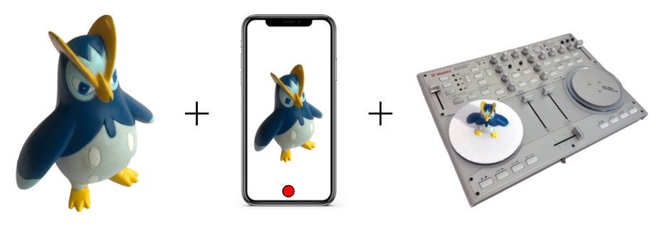
For our implementation, we chose a method that approximates the latter – the turntable method. We will start with a subject (a toy figurine), a smartphone camera to take photos of the subject, and a means of rotating the toy.
Check out the project video to get some more in depth information on these techniques.

The object was chosen for its simple form. The choice of a simple iPhone camera allows for simple calibration openCV, since we can grab crucial sensor information from the manufacturer. A turntable was needed, and we had a digital one with two wheels on hand. A simple setup.

The object will be placed on the turntable, with the camera in a fixed position to the side. The object will be rotated, with the camera capturing a photo of the object every 𝞱 degrees of rotation to create a series of photos around the subject.
If we imagine, instead, that the camera is rotating around a stationary object, then we can lay out this diagram of known dimensions.
With a known 𝞱 degrees between rotations, we can calculate the distance T between cameras. The distance d from the center of rotation to the camera is measured manually when setting up the apparatus. We know the camera position at each interval. The focal length f and other intrinsic camera parameters are calculated with calibrations.

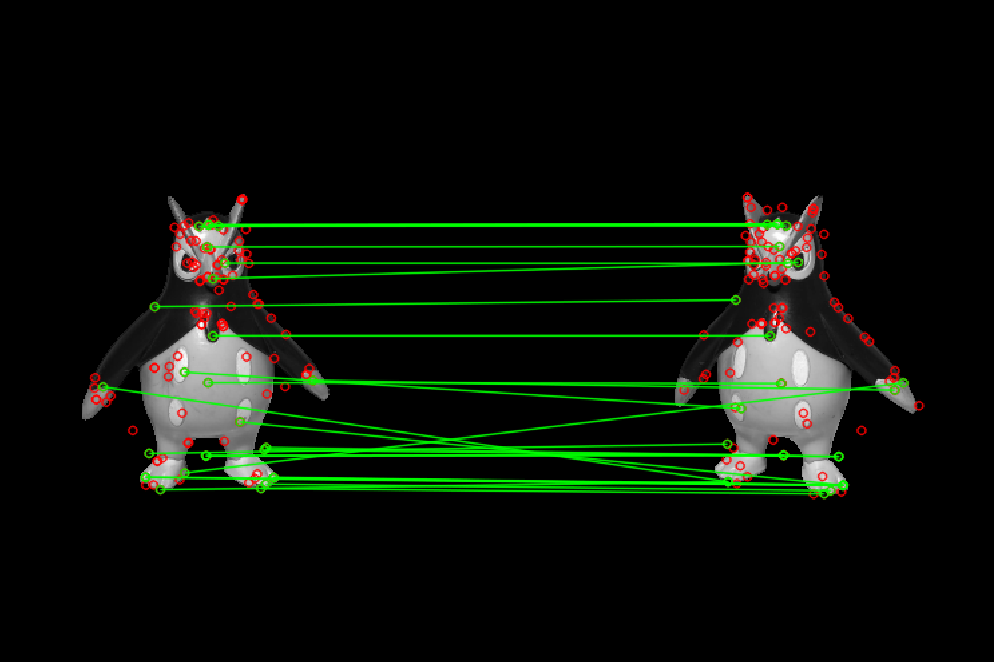
We will first need to calculate and identify matching keypoints for each pair of images. We will first find the keypoints and descriptors for each image – this will utilize the SIFT algorithm. Then, we can use a matching algorithm (eg. Brute Force) to first find all possible matches. Then, we will determine a threshold to filter for good matches.
Visualizing as a diagram on the turntable, these matching keypoints represents features that a pair of cameras has identified as being the same elements from different perspectives. We can use the difference between their location in the image plane to determine the feature’s depth – much like how our eyes function.


Once we have its real world coordinates we will be able to construct an equation for a line from the camera’s position to this point of intersection. The lines from each camera will intersect with each other at the matched point on the 3D object. Thus using both line equations we’ll be able to find the original 3D point to be added to the point cloud.
The Algorithm.
Taking images
Turntable setup with iPhone camera and wheel.
Camera Calibration
Use openCV chessboard functions to determine camera parameters.
Undistort Images
Use camera parameters to undistort images from lens distortion.
Identify Features
Determine image keypoints and descriptors using SIFT algorithm.
Feature Matching
Match features from image pairs using Brute Force.
Triangulate Feature Depth
Calculate feature position in 3D world space using image plane difference.
The Results
To set up the apparatus, we used an actual turntable as a rotating platform (because it was convenient). A paper wheel was added with degree markings for easy rotation reference.


With the turntable apparatus set up, we placed the toy on the rotating platform and took pictures for every 20º increment. This generated 18 evenly rotated photos around the Toy.

Processing Images.
Utilizing the SIFT algorithm, we realized a drawback of keypoint detection. Since keypoint detection relies on patches where gradients of the images are unique. This most often occurs on the edges between color changes.
As a result, the matches selected are dense in detailed areas (ie. the facial features), but less dense in areas of flat color. As such, the resulting sparse point cloud lacks definition on these regions.
These errant ”noise” points can mostly be attributed to ”noise” in the original images. Since the Turntable setup was by no means professionally constructed, there were consistent noise across the images’ backgrounds. This caused keypoints to be detected and matched away from our target.

These stationary elements can be seen in the ”halo” of points of above the Toy, and in the cloud surrounding it. This also includes the angle markers on the Turntable platform itself, which was printed to aid in controlling the rotation: these markers were also detected across the images, which accounts for the ”halo” of points below the Toy.

Output Point Cloud.
This is a 360 view of the point cloud of our Toy as processed through our algorithm without removing erroneous points.
The noise in the previous image can be seen in 3D space, cluttering the desired point cloud. The halo below the object is especially apparent.

Final Point Cloud.
This is a 360 view of the point cloud of our Toy as processed through our algorithm and erroneous points cleaned.
We can remove all points that we would not expect in the model – noise above and below the object, and points outside of the cylinder of space demarcated by the wheel.
